Chaldni Patterns
Interactive simulations
By Juan Carlos Ponce Campuzano, 03/June/2022
Open the Controls to change parameters or modify the size of the plate and the color of the particles. You can also save your favorite Chladni pattern.
Historical background
We now know that sound propagates in waves through a solid, gas, or liquid medium — but we didn't always know this. In the late 1700s, the German scientist Ernst Chladni was the first to show that sound travels via waves by devising a way to visualize their vibrations.

Image in the public domain in the
United States, via Wikimedia Commons.
One of Chladni's best-known achievements was inventing a technique to show the various modes of vibration on a rigid surface. When resonating, a plate or membrane is divided into regions that vibrate in opposite directions, bounded by lines where no vibration occurs (nodal lines)
Chladni's technique, first published in 1787 in his book Entdeckungen über die Theorie des Klanges ("Discoveries in the Theory of Sound"), consisted of drawing a bow over a piece of metal whose surface was lightly covered with sand. The plate was bowed until it reached resonance, when the vibration causes the sand to move and concentrate along the nodal lines where the surface is still, outlining the nodal lines. The patterns formed by these lines are what are now called Chladni figures.

Image in the public domain in the
United States, via Wikimedia Commons.

Mathematical model
The deformation of an elastic plate under an external force was a very difficult problem and there were many attempts to solve it. It was until 1850 that the definitive breakthrough was achieved in a long article by G. Kirchhoff in the form of the differential equation
To know more details about the solution of this problem and its history, I recomend to consult the following paper From Euler, Ritz, and Galerkin to Modern Computing by Martin J. Gander and Gerhard Wanner.
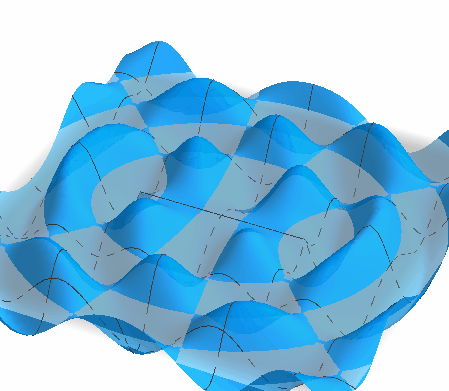
Chladni pattern in 3D
How this simulation works
One way to approximate Chladni figures is by using sine and cosine functions. In particular, this simulation shows an unclamped plate with a finite number of sources $A_i = (x_i, y_i)$. This is a simplified model approximated with the function
If you find this content useful, please consider supporting the work using the links below.
References
- Martin Skrodzki, Ulrich Reitebuch, and Konrad Polthier (2016). Chladni Figures Revisited: A Peek Into The Third Dimension Bridges Finland Conference Proceedings pp. 481-484.
- Martin J. Gander and Gerhard Wanner (2012). From Euler, Ritz, and Galerkin to Modern Computing SIAM Review Vol. 54, Iss. 4.
- G. Kirchhoff (1850). Über das Gleichgewicht und die Bewegung einer elastischen Scheibe. Journal für die reine und angewandte Mathematik Volume: 40, page 51-88.